Moduli Regularization
This post is a brief, intuitive summary of my paper, “Geometric sparsification in recurrent neural networks.” Academic publications emphasize formal descriptions of methods (for good reason!) in a way that isn’t always the most useful for readers attempting to simply learn the ideas being proposed by a paper. My goal in this post is to offer a more friendly description of the ideas in my and my collaborators’ paper. The main goals of our paper are:
- To show that RNNs have natural, intrinsic geometric structure;
- To show that knowledge of this structure allows us to create more efficient neural nets;
- To bypass the necessity of foreknowledge, and learn the ideal geometric structure during training.
Fixed moduli regularizers
Our theory, a version of the manifold hypothesis, is that most data is nicely organized along hidden, latent manifolds. We specifically focus on the special case of recurrent neural nets (RNNs). Recurrent neural nets are neural networks designed to deal with sequential data, such as the words in a sentence, or EEG readouts over time. They take their output at time \(t\), and the sequence input at time \(t+1\), as two inputs to compute the time \(t+1\) output. In principle, this function can be any manipulation on \(\mathbb{R}^n\), but I’d suggest thinking of this as, for instance, a state space for a physics problem, or a continuous approximation of a discrete space.
In essence, recurrent neural nets are discrete approximations of differential equations, which have fixed stable loci. So, here’s a natural question: if you knew beforehand what the state space of a recurrent neural net was, would this let you design a better RNN? The word “better” here needs investigation: this could mean more accurate, but it could also mean more efficient, or simply faster to train. We didn’t manage to find a way to simply improve the total quality of the neural net using foreknowledge of the state space geometry: the wonderful think about neural nets is that they’ve very good at figuring out these complex structures, when you give them access to enough dimensions! However, another axis on which you can improve a neural net is its sparsity: that is, how many of the matrix entries can be set to 0. Multiplication is the most expensive (in terms of computation time and energy) operation that neural nets regularly conduct. Moving to multiplication by sparse matrices allows us to avoid a lot of these costs. We found that we could leverage foreknowledge of the state space to create networks that are more resilient to sparsification, which is the main result of our paper.
Again, let me present intuition before equations: suppose that the state space of an RNN is the abstract manifold \(M\). There are an infinite number of ways that \(M\) can be realized as a subspace of \(\mathbb{R}^n\), when \(n\) is sufficiently large (twice the dimension of \(M\) is sufficient, this is the Whitney embedding theorem), which all can plausibly function as equally effective latent spaces for the RNN. There won’t necessarily be any distinction between the abilities of different embeddings of \(M\) to approximate the true dynamics problem the RNN is attempting to solve. However, different embeddings of \(M\) will require different numbers of parameters to specify position on \(M\). For example, suppose the state space of our RNN is the circle \(S^1\): this can be expressed perfectly using only two nonzero dimensions in \(\mathbb{R}^n\) as \((\cos(\theta), \sin(\theta), 0, 0, ..., 0)\). However, it can equally be embedded as \((\cos(\theta), \sin(\theta), \cos(\theta), \cos(\theta), ..., \cos(\theta))\), which necessitates far more tracking of variables and computations.
An optimally sparse representation of a manifold \(M\) is just the set of points \(x \in M\). Any point \(x \in M\) can (of course!) be represented simply by \(1 \cdot x\), and \(0 \cdot y\) for \(M \ni y \neq x\). Tragically, our computers don’t have infinite memory banks. However, we can do a good approximation to points in a compact manifold just by taking a good discretization. We’ll tell the RNN that we want this by regularizing the weight update matrix.
 |
|---|
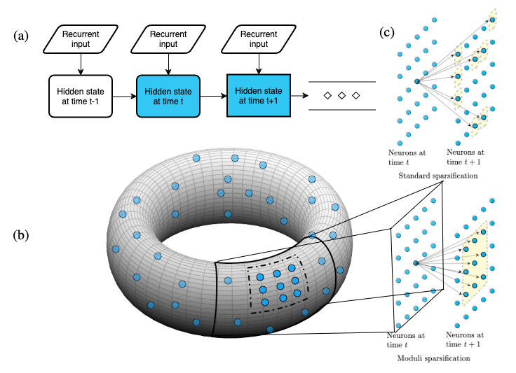
| Figure 1 from our paper. (a) Shows the structure of an (Elman) RNN. (b) Hidden state neurons, represented by blue dots, are embedded into a moduli space, the torus. (c) Sparsification of the hidden update matrix of an RNN. Above depicts random sparsification, and below depicts sparsification in line with moduli regularization (briefly, moduli sparsification). Yellow boxed points are neurons with a non-zero weight connecting them to the center neuron. Moduli sparsification respects the geometry of the chosen moduli space, which is ignored by standard sparsification techniques. |
A diagram displaying what’s happening in the model is shown above: our plan is to force the RNN to look like diffusion on a manifold. In equations, we do this by choosing embeddings of the neurons \(i: \{1, 2, ..., n\} \to M\), and including a regularization term which punishes the neural net for deviating from the metric structure on $M$. In equations, this is a penalty
\[R_f(W_{hh}) := \sum_{j,k} f(d_{M}(i(j), i(k)))|w_{jk}|^\ell,\]where \(W_{hh} = (w_{jk})\) is the weight update matrix of the RNN, \(d_M\) is the distance function on \(M\), \(\ell\) is a nonnegative integer, and \(f: \mathbb{R}^{>0} \to \mathbb{R}^{>0}\) is a function, chosen as a hyperparameter. Taking \(f(x) = x\) will yield an example like the figure shown above, for example. The mathematical details here aren’t really important, though: it’s clear that something will work, and the important idea is just that things like we show in the lower part of the figure are good, and and things like the upper part are bad.
Our paper proceeds to show that this idea has merits in the sparse regime, using very reasonable control experiments. You can read the paper for details. However, there’s a big, hanging question: what do we do when we don’t know state space for the RNN? One surprising result that we present is that, in complex cases, lots of different manifolds work well, and tend to work better than reasonable alternatives. Simply picking a random manifold will work ok. This is surprising and interesting, but not a satisfying resolution to the question. So let’s present a better idea: we can learn the manifold \(M\) during training.
Learned moduli spaces
You’ll recall that part of the set up for our regularization scheme was choosing, essentially as a hyperparameter, a list of manifold embeddings \(i: \{1, 2, ..., n\} \to M\). When \(M\) is a smooth manifold and \(f\) is differentiable, we can actually think of this as a parameter of our network, however, and compute gradients of the loss function! (If you aren’t familiar with manifolds, nothing will be lost by simply assuming \(M\) to be \(\mathbb{R}^n\), which is the relevant use case regardless.) If we update these gradients along with the gradients of the traditional weights of the RNN, we will move from random embeddings in \(M\) to an embedding that’s optimized for the specific problem. In principle, if \(M\) is simply a high dimensional Euclidean space, it’s possible to learn an optimized approximation of the RNN’s state space in an end to end manner using this technique! This completely avoids the difficulty of choosing the manifold \(M\) and embedding \(i\) as hyperparameters of training.
There are some math details here: I earlier encouraged simply ignoring the function \(f\). However, if \(f\) is set to be the identity function, the regularizer will simply destabilize itself, choosing a single point as the `optimal’ moduli space. In our paper, we chose an inverted difference of Gaussians
\[f(x) = c - c(e^{-\frac{x^2}{\sigma_2}} - e^{-\frac{x^2}{\sigma_1}})\]to overcome the collapse, where \(c, \sigma_1, \sigma_2\) are hyperparameters. Again, however, this equation doesn’t require serious exploration: the point is simply that information should diffuse around the manifold, but also that neurons must repel each other at least a little bit to avoid collapse.
You should have some concerns about this method: we’ve not only added a bunch of trained parameters to our network, but we’ve also materially complicated our gradient calculations and added overhead calculations of turning the model parameters into distances that can be used for regularization. In practice, however, the additional costs are small: for simple manifolds like \(\mathbb{R}^d\), the distance function is quick to calculate, and we’re not actually adding that many parameters: again, taking \(M = \mathbb{R}^d\) and an \(n\) dimensional hidden space in the RNN, we are adding \(nd\) trained parameters. However, the weight update matrix by itself has \(n^2\) trained parameters, and it’s reasonable to expect we will choose \(d << n\). In practice, the additional computations were marginal in our experiments.
Conclusion
We introduced an end-to-end manifold learning technique for RNNs. This is intrinsically interesting! It also is potentially useful, if you are trying to write a very efficient RNN. Really, though, we should be taking this as intuition about the way RNNs work, and as a foundational technique for manifold learning in neural nets. RNNs are the most natural application, which is unfortunate because they are no longer in vogue. Socially impactful generalizations will involve bridging this technique to new architectures, particularly transformers.
However, RNNs are still used in some reasonable, practical cases, and the technique itself is, I hope you will agree, an interesting idea! I’d encourage you to look at our paper if you’d like to see the efficacy of moduli regularization on practical problems.