Residual expansion: hyper-connections, virtual width, and attention in the depth direction

There have been quite a few interesting takes on what I’m going to call “residual expansion” over the last year, particularly notably Deepseek’s Manifold-constrained Hyper-connections. Residual expansion is a new axis of sparsity introduced to any residual network structure, notably transformers in NLP, which is also where all experiments in the papers I reviewed were conducted. It’s particularly exciting as a way to access more information and more precise compute in the transformer architecture without simultaneously scaling the actual energy/memory demands of the system.

The expositions in some of the relevant papers can be quite different, though, so I wanted to work out the math to evaluate the real differences between the different approaches to residual expansion. Specifically, I’ll be looking at (manifold-constrained) hyper-connections, virtual width networks, and residual matrix transformers. These notes are primarily for my own benefit as I think through the methods, but I will try to keep them relatively accessible. Organizationally, I’ll briefly go over the prerequisites and motivation for residual expansion, then discuss the three approaches.

Background: residuals, transformers

The super-deep networks common today reflect several clever improvements to neural architectures over the last couple of decades, notably ResNets breaking the barriers on deep convolutional networks. Essentially, the problem is vanishing gradients: when you’re training a neural net, weights are changed through back-propagation: the loss function tells us how well the network approximated a given batch of data, and we take the derivative of the loss function with respect to each parameter in order to update that parameter. If our set-up is good, we’ll then take small steps in the direction of the gradient to improve our network.

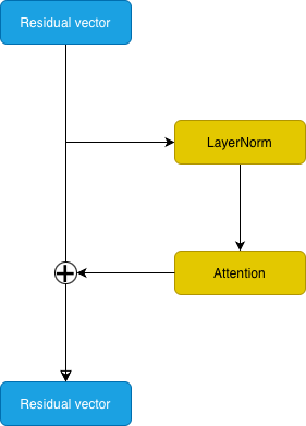
There’s a problem though: the chain rule means that the downstream effect of parameters in early layers is multiplied by the gradients of all downstream parameters, which means if the gradients on the final layers are small, the gradients on early layers will be multiplied by small numbers, and therefore updated by less than we likely want them to be updated by. There are a lot of hacky solutions you can try to do to fix this: layer-wise gradient scaling is an obvious choice, or just using shallow networks. ResNet’s approach is architectural, but essentially, the idea is to set up the network so that each layer is initialized close to the identity matrix, so that gradients will propagate easily to early layers of the network. Instead of having each layer of the network calculate the input to layer \(t+1\) as \(x_{t+1} = N_t(x_t)\), we set \(x_{t+1} = x_t + N_t(x_t)\). \(N_t\) can be anything, but is generally a self-contained block: convolutional layers in ResNets, layer norm + attention, or layer norm + MLP in transformers are common examples. This is a simple idea, but it allows us to train much larger networks.[^1]

Instead of layers transforming the input value, the residual vector is edited by each layer of the network. Apply normalization first for best results.

Motivation: Sparsity, conditional compute, superposition

One of the really big updates to transformers over the last few years is Mixtures of Experts (MoE): while it’s hard to be sure with large proprietary models, it’s likely that all major NLP transformers being trained today use them. The idea isn’t so complicated: with any LLM, a lot of information is being stored in the weights of the network, but a lot of that information is completely irrelevant to any given task. For example, if I ask an LLM about Napoleonic history, it still is multiplying my query by everything it knows about calculus, which is an awful waste of compute.[^2]

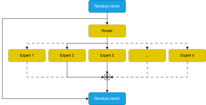
Mixture of experts suggests that, instead, we train a large array of experts (generally MLPs) for each MLP layer, and use a router to decide which experts to use for any given query. This comes with some engineering complexities, but mathematically it’s pretty simple: a router network \(r\) takes the residual input \(x\) and outputs a distribution over a set of experts (generally MLPs) \(\{E_1, E_2, ..., E_m\}\), a subset of which are then used by the model. A common implementation is

\[MoE(x) = \sum_{i \in \operatorname{argtop-k} \{r(x)_i\}} r(x)_i E_i(x).\]

I illustrated this in the figure below. This turns out to be sort of a free lunch: obvioiusly, if it works nicely, it’s going to solve our Napoleon/calculus problem. It also lets us add a lot of parameters to our network without increasing the compute per sample requirments, and network quality continues to scale with total parameters, not just the number of active parameters!

| | [:–:] |The Mixture of Experts uses a router to choose specific experts to process the input—in this example experts 2 and 3. The other experts are inactive on this input.|

One concern I had when I first learned about MoEs was that it would take much longer to train an MoE network: since they have such high sparsity, most of the weights in most of the experts are not being changed on any given training sample, so we might expect to need a lot more data for an MoE to train. In fact, this isn’t the case: larger networks usually train faster and better on the same token budget as small networks, and MoEs are no exception: they train faster and better than traditional transformers with the same number of active parameters. Which is pretty crazy! The take-away is that sparsity in your network is a powerful tool for scaling.

Another motivation I wanted to touch briefly on comes from interpretability research. The so-called superposition hypothesis suggests that the residual stream of the transformer is a sum of many different, potentially interpretable, components, which are packed into the residual stream. Having a larger residual stream allows you to store more components—but most of those “directions” are being used by only a few, specific updates. If we take as given that the residual stream really should be thought of as being a sum of sparse things, and that MoEs seem so miraculous on the sparsity axis that is knowledge, we can reasonably hope that there’s some way to introduce useful sparsity to the residual stream itself.

Residual expansion: outline

The total parameters of a transformer scales quadratically with the dimension of the residual stream. Our goal, as outlined above, is to modify the way that the residual information is fed into generic blocks (generally, attention and MoE blocks) to allow us to expand the residual space, but not change the parameters required for the generic network blocks.

A pretty generic approach to this is for a block \(T\) to be applied to residual vector \(x_t \in \mathbb{R}^N\) at the cost of a residual vector \(\hat{x}_t \in \mathbb{R}^n\), \(n < N\), via

\[x_{t+1} = A_{res} x_t + A_{up} T(A_{down}x_t),\]

where the \(A_{res} \in \mathbb{R}^{N \times N}\) and \(A_{up}, A_{down}^\top \in \mathbb{R}^{N \times n}\). As written, this approach doesn’t really get you much in compute savings: we’ve decreased the cost of the block \(T\), but by adding in the potentially costly \(A_{res}, A_{up}, A_{down}\) matrices. To become compute efficient, we need to structure the \(A\) matrices to be sparse and highly structured.

(Manifold-constrained) Hyper-connections

Hyper-connections are the most straightforward approach to this expansion: essentially, we add a channel dimension to the residual tensor, \(x_t \in \mathbb{R}^{C \times n}\), where \(C\) is the expansion factor. This gives a particularly nice form for the \(A\) matrices we introduced above: we can set \(A_{res} \in \mathbb{R}^{C \times C}\), and \(A_{up}, A_{down}^\top \in \mathbb{R}^{C \times 1}\). Generally, \(C\) will be something small: \(C = 4\) was used in most of Deepseek’s experiments.

Aside. A huge trend in modern research is making as many parts of the network be functions of the input as possible. There’s lots of reasons this might be good, but maybe the simplest is that it’s tricky for MLPs to do multiplication, but multiplication is pretty great, and gate layers give the network much better ways to do multiplication. So in gritty implementation details, the \(A\) matrices won’t directly be network parameters, but rather \(A_i = c_i \operatorname{tanh}(\theta_i \hat{x}) + b_i\), where \(\hat{x} = \operatorname{LayerNorm}(x)\) is scaled input data. The trained parameters are \(\theta_i\), \(c_i, b_i\), with the latter two scalars.

Ablations show that all components contribute to the final network improving. While this is a good idea on its face, it does introduce some interesting instabilities to the network: the \(A_{res}\) matrix has taken the place of the identity matrix. As discussed above, letting the residual take the form \(x_{t+1} = x_t + T(x_t)\) helped stabilize gradient propagation during training. If \(A_{res}\) gets too small we could have the same gradient issues we had without the residual connection at all. Therefore, and this is where the manifold with boundary comes in, we should normalize \(A_{res}\) to be double stochastic: have rows and columns sum to 1.

This is equivalent to lying somewhere in the polytope of permutation matrices, and Deepseek proposed using the Sinkhorn-Knopp algorithm to normalize \(A_{res}\) to be doubly stochastic (rows and columns sum to 1, all entries nonnegative), greatly improving stability. The Sinkhorn-Knopp algorithm is an iterative algorithm that alternately scales rows and columns to sum to 1.

Aside. Instead of Sinkhorn-Knopp, a recent paper suggested that it was better to directly calculate coefficients on a linear combination of permutation matrices. Unlike finite iterations of Sinkhorn-Knopp, this actually ensures the resultant matrix is doubly stochastic, and when \(C\) is small, like \(C=4\), it’s very efficient. (I imagine this approach won’t really scale well much past \(C=4\), though, since it will scale with \(C!\).)

Virtual Width Networks

The idea for virtual width networks (VWNs) is essentially identical to hyper-connections: while hyper-connections have integer scaling factors, a reasonable question (from a mathematical perspective) is whether this can be generalized to arbitrary rational scaling factors. From a practical perspective, we might also think that the hyper-connections set-up is a bit limiting: every layer \(T\) access a 1 dimensional slice of the channel set. While this is convenient to write, it’s pretty far from how wonderfully mixtures of experts partitioned information. We would like something that allows us to flexibly choose which information to give layer \(T\) with much greater granularity.

VWNs argue first that we should be projecting our channel dimension into more than a single dimension. (Here I depart a bit from the exposition in the VWN paper, so check it out for a description that might work better for you.) Keeping the notation from above, let \(x \in \mathbb{R}^{C \times n}\) be an expanded residual space, which we can view as a set of \(n\) vectors of dimension \(C\). We’ll be compressing to a vector \(\hat{x} \in \mathbb{R}^{C \times m}\), with \(m < n\). The scaling factor of the expansion is \(\frac{n}{m}\).

Instead of operating on the \(C\) dimension, I think it’s nicer to view \(A\) as acting on the \(n\) dimension, so we’ll have our matrices \(A\) act on the right in

\[x_{t+1} = x_tA_{res} + T(x_tA_{down})A_{up},\]

with \(A_{res} \in \mathbb{R}^{n \times n}\), \(A_{down}, A_{up}^\top \in \mathbb{R}^{n \times m}\). We’re compressing the information of \(n\) vectors in \(\mathbb{R}^C\) into \(m\) vectors in \(\mathbb{R}^C\) by (weighted) averaging them together using the matrix \(A_{down}\), and similarly for \(A_{up}\) and \(A_{res}\).

One way to view this transformation is to think of the \(A\) matrices as being something like attention matrices in the depth direction. The layer hyperparameters set which of the \(n\) vectors, and in what combination, are most relevant for layer \(T\). We finally unfold \(xA_{down} \in \mathbb{R}^{C \times m}\) to be a \(mC\) dimensional vector.

This recovers hyper-connections as a special case where \(m = 1\), obfuscated a bit by my choice to swap which side the \(A\) matrices were being applied to. (Sorry!)

Aside. As in hyper-connections, the matrices \(A_i\) will be functions of the input \(x\), with very similar parameterizations.

Residual matrix transformers

Residual matrix transformers (RMTs) carry along the analogy of attention in the depth direction introduced by VWNs. However, RMTs are no longer generic expansion and contraction techniques for any network block: they are specific modifications to the transformer designed to operate with a larger residual—a matrix residual—and smaller attention/MLP blocks.

Let’s revisit the way that models interface with the residual stream: generally, some normalization is applied to the residual vector, then a matrix (e.g. the QKV matrix) is applied to get new vectors for downstream tasks. The mathematical recipe is one matrix plus one vector gives you a new vector, and these costs are baked into the transformer. So, instead of trying to keep the matrix of the attention/MLP layers, RMTs expand the residual to be a matrix, and replace the layer \(T\)’s input matrix with a vector. Let’s do the attention layer explicitly: the residual \(X\) is a matrix, then

\[MHA(X) = \sum_h w^O_h \otimes SHA(X),\]

where \(SHA(X) = \operatorname{softmax}(Q^\top K/\sqrt{d})V\), where \(Q^{(h)} = q^{(h)} \cdot X\) is the evaluation of a vector \(q^{(h)}\) on the matrix \(X\), and likewise for \(K, V\).

I usually think of the residual as being a square matrix, but there’s no mathematical requirement that it be so, giving a similar flexibility as hyper-connections have, while decreasing the number of trained model parameters. A good connection to make here is with linear attention (and broadly, Hopfield networks), as the idea is very similar: we update a matrix information storage system with low rank additions, and this compresses information more favorably than a vector based memory system does.

We’ve already noted that VWNs are a generalization of hyper-connections. But where do RMTs fit into this mix? They don’t have a totally obvious parallel: they don’t even fit into the general sparse \(A\) matrix formalism we introduced at the beginning. But there should be a connection in there.

Math aside: pulling apart RMT

Let’s focus on \(A_{down}x\), in the case of hyper-connections, specialized so \(C=n\) (so \(x \in \mathbb{R}^{n \times n}\), where we are with RMTs). \(A_{down}\) is a \(1 \times n\) matrix, aka a vector, and the multiplication \(A_{down}x\) is an \(n\) dimensional vector, equal to the evaluation of the matrix \(x\) on the vector \(A_{down}\). This is evocative of the RMT formulation, except that it’s using the same \(A_{down}\) for the entire layer, rather than specialized projections for each component. Ignoring layer norms, the query vector (multiplying on the right for convenience) will be \((A_{down}x)Q\). Expanding this out for the (single head) attention matrix calculation

\[\operatorname{Att} = \operatorname{softmax}(A_{down}xQK^\top x^\top A_{down}^\top / \sqrt{d}).\]

In contrast, the RMT formulation of attention will have

\[\operatorname{Att} = \operatorname{softmax}(q \cdot x x^\top \cdot k^\top /\sqrt{d}).\]

While doing similar things, it’s clear that neither version fully encapsulates the other: they differ by a single non-commutative operation of replacing \(A_{down}x Q\) with \(A_{down}Qx\) (and similar for keys, values). Arguably, the standard hyper-connections formulation allows greater flexibility, as \(A_{down}\) is a function of \(x\), while \(q\) in RMT is a fixed parameter of the network without \(x\) dependency, though this could be altered without much difficulty. I don’t see any a priori way to compare these, so it might just come down to experimental results.

Footnotes

[^1] The convolutional setting is a little more complicated, since convolutional networks are often simultaneously increasing the number of channels and decreasing the height/width of the data, so we can’t necessarily assume \(x_{t+1}\) and \(x_t\) have the same shape. I haven’t double checked, but I believe that ResNets just use a \(1 \times 1\) strided convolution to change the shape of \(x_t\) in this case, but that’s still much lighter than \(N_t\) generally is. Incidentally, this can also be viewed as motivation for some of the additional ideas used in hyper-connections! But generally, transformers greatly simplify the setting, as the attention and MLP layers are designed intentionally so that \(x_{t+1}\) and \(x_t\) have the same shape.

[^2] You could also argue that it is biologically implausible—as has been much harped on over the last decade, humans are never using more than a small fraction of their brain at any given time! But biological implausibility is a sort of so-so argument: while it can be good inspiration and good to think about, I never view it as dispositive.