TTT is not linear attention—but it might be something weirder

An interesting paper by Liu et al. came out last week, arguing that we should reconceptualize the variety of test time training (TTT) with KV-binding architectures don’t actually bind keys and vectors—and perhaps could therefore be thought of as another form of linear attention. The paper included a lot of interesting experiments, and I think raises several important questions. However, ultimately I don’t think I quite believe the case that Liu et al. make, or their interpretation of all listed results. Rather, I think that TTT has several surprising properties that make it look different from both linear attention and full attention. To develop the case, I wanted to perform a detailed exploration of Liu et al.’s paper.

This post does presume some familiarity with Liu et al.’s paper, as I don’t intend to fully recapitulate their results. It’s a fascinating case study, and well worth a read.

Brief background: Attention, Linear attention, and TTT with KV-binding

Let’s start by looking at scaled dot-product multihead attention, as implemented in transformers. Multihead attention is a sequence mixing function, often written as \(\operatorname{softmax}(QK^\top/\sqrt{d}) V.\) Personally, I think that the batched/matrix form is a lot trickier to think about than the unbatched form, so let’s unroll this for a decoder transformer evaluated specifically at token \(t.\) In that case, the update at index \(t\) is \(\sum_{i \le t} a_i v_i,\) where \(a_i = \operatorname{softmax}_i(\{q_t \cdot k_j\}_{j \le t}).\)

There are two different interpretations of this, both of which are productive and lead to interesting ideas! First, what I will call the linear attention direction, focuses on my unrolled formulation of attention as \(\sum a_i v_i.\) We know that the attention scores \(a_i\) are computed with a (infinite dimensional) kernel via the softmax. But what if instead of applying softmax, we applied a finite dimensional kernel to calculate the \(a_i?\) The simplest finite dimensional kernel is just the dot product, so let’s focus on that. If \(a_i = q_t \cdot k_i = q_t k_i^\top,\) then we can rewrite our attention update as \(\sum a_i v_i = \sum (q_t k_i^\top) v_i = \sum q_t (k_i^\top v_i) = q_t \sum k_i^\top v_i.\) Importantly, we no longer have to keep our cache of keys and values in order to operate attention: at inference time, we can just remember the sum \(\sum k_i^\top v_i\)! This was originally observed by Katharopoulos et al. in their famous “Transformers are RNNs” paper. Many forms of linear attention work from essentially this standpoint, plus lots of architectural improvements.

Another direction you can go is to zero in on the batched formulation of attention. Again specializing to token \(t\), the update is given by \(\operatorname{softmax}(q_t K^\top) V.\) This can be thought of as some abstract function \(f(x) = \operatorname{softmax}(x K^\top) V.\) The function \(f\) in attention is non-parametric and non-linear, determined by the fully history of observed tokens. The natural question is: Is there any other way to construct a non-parametric, non-linear function? Proposed by Sun et al., test time training answers this question in a very machine-learning way: we want to construct a nonlinear function, so let’s use gradient descent! We can initialize a function \(f\) as a neural network with parameters \(\Theta.\) Then, given a history of keys and value vectors, we can train \((f, \Theta)\) using a surrogate loss function—in the literature, this is frequently something like \(\sum \frac12 \mid \mid f(k_i) - v_i\mid \mid^2.\) If you specialize to the case where \(f\) is a linear function, this unsurprisingly recovers something that looks a lot like linear attention. But we’ve gained quite a bit of flexibility, since \(f\) is no longer required to be linear, but also doesn’t grow in proportion to the sequence length. Having multiple sets of parameters updated at different times can be confusing—the standard notation here is to refer to the network as computed by “outer loop” parameters that are updated during training and frozen at test time, and “inner loop” parameters that are flexibly updated at test time. You can think of the inner loop parameters as being sort of like an attention matrix, in that they depend on the inputs, but are used like a matrix.

Or at least, that’s the idea—but Liu et al. think otherwise, so let’s go into the paper!

In theory: gradient descent looks a lot like linear attention, but mind the gap

One of the key inspirations behind many TTT architectures is the update made in linear attention. Since attention works so well, we model the loss function according to roughly what we think attention does: if a query activates a key, make the corresponding value vector have a proportionally greater output.

Liu et al. write this out in Theorems 5.1-5.3, but make a stronger argument: not only is the nonlinear function \(f\) inspired by linear attention, its updates can be interpreted as a specific form of linear attention. I’ll focus on Theorem 5.1. Liu et al. rewrite \(f_\ell(x) = W\ell \phi_\ell(x),\) where \(W\) is the final linear projection of the neural net \(f,\) and \(\phi\) is everything else, and \(\ell\) is the number of gradient descent steps taken. The essential argument of the theorem is that we can rewrite the final output after a single gradient descent step on input data \((k, v)\) as \(o = (W_\ell + \phi_\ell(k)g_\ell(k, v)) \phi_{\ell+1}(q),\) where \(g_\ell(k, v)\) is the gradient. In particular, the update to \(W_\ell\) looks like linear attention, where the proxy key \(\hat{k} = \phi_\ell(k),\) the proxy value is the gradient \(\hat{v} = g_\ell(k, v),\) and the proxy query \(\hat{q} = \phi_{\ell+1}(q).\)

I’m not convinced this is a meaningful claim though! There are several noticeable gaps in the argument:

• The update to the output isn’t determined fully by the gradient change to \(W_\ell,\) note that we also used \(\phi_{\ell+1} = \phi_\ell - \nabla \mathcal{L}\) in computing the output, meaning we did a step of stochastic gradient descent on an arbitrarily shaped neural network, and prepended that step before applying multiplication by \(W_\ell.\) It doesn’t matter if \(W_\ell\) updates like linear attention does when the the rest of the nonlinear network updating also matters.
• Even though the update to \(W_\ell\) superficially looks like linear attention, it’s really worth pointing out the ways in which it differs. Using the proxy key/proxy value terminology, the proxy key \(\hat{k} = \phi_\ell(k)\) is calculated by a nonlinear network whose coefficients are a function of the past data. You cannot obtain the same realization in a standard linear attention setting, where the key vector $k$ is a linear function of the input that does not depend on prior token values. I find the case for the proxy gradient \(\hat{v}\) suffers similar challenges.

I think there’s a fairly clear breakpoint between linear attention and TTT, and it’s exposed quite well by Liu et al.’s paper: in linear attention, like standard attention, the query, key, and value are all functions of the outer loop parameters and the current token value \(x_t\). The proxy query, proxy key, and proxy values constructed by Liu et al. don’t satisfy that condition: these proxy values are a function of outer loop parameters, but also of inner loop parameters. Since inner loop parameters are themselves a function of past tokens, \(\hat{q}, \hat{k},\) and \(\hat{v}\) depend on \(x_i\) for all \(i \le t.\) This dependence fundamentally breaks the proposed analogy. This is also why TTT doesn’t really parallelize over the sequence direction, which is the most serious efficiency problem TTT faces.

In practice: reviewing the evidence for TTT not behaving like attention

I think this part is the most interesting part of Liu et al.’s paper, and the reason I wanted to do a deep dive on it. They perform a number of fascinating ablations which shed a lot of light on TTT—things that probably should have been studied before! That said, while I think all of their experiments are interesting, I don’t think any of them prove that TTT is linear attention—rather, I think they expose surprising traits of the TTT system.

4.1: Increasing gradient steps leads to worse performance

This is an interesting and surprising result, and I think the strongest put forward in the paper. By increasing the number of gradient steps taken by the inner loop, we can decrease the inner loop’s proxy loss, achieving what is hypothetically a better outcome than if we take only a single gradient step. But in practice on pretrained networks, increasing the gradient steps improves the self-supervised proxy loss, but results in worse downstream performance.

This is powerful and interesting, but I don’t think it’s a death knell for TTT. Let me give an analogy: suppose you trained an RNN, but during training you only ever exposed it to a single update step. In principle, if the network updates its hidden state correctly for any single step, it can work for arbitrary sequence lengths. In practice, it’s important to compute loss at a large variety of sequence lengths to achieve generalization—and even then, you can’t necessarily expect the RNN to generalize beyond the longest sequence length it was tested on.

Ultimately, I think this experiment demonstrates that TTT similarly doesn’t generalize in iteration directions beyond its training data. From an outer loop perspective, the key and value vectors used in the proxy loss were tuned specifically to the single-gradient-step setting—in fact, to train the key and value vectors, they specifically see a loss function of a single gradient step, if that’s what they’re trained on! We shouldn’t necessarily assume that the same key and value vectors are optimal when we move outside the training distribution by taking multiple gradient steps.

Aside. I think this is a reasonable refutation, but I want to emphasize that I came up with it only after seeing the experiments of Liu et al., and I would not necessarily have expected them. So take it with an appropriate grain of salt.

4.2: TTT with gradient ascent

The precise claims in the paper for the next few sections were a little ambiguous, so I reached out to the authors who very kindly clarified the experiments conducted here. All experiments on modifying the TTT algorithm were done by training fresh models, not by directly modifying the gradient interactions in pretrained models.

I don’t think that this result is particularly surprising! As the authors note, using gradient ascent with loss functions like the Frobenius inner product are the same as multiplying the loss by negative 1—or similarly, the value vectors by negative one. In particular, since the outer loop gets to choose the key and value vectors, these negative ones can be absorbed into the outer loop. Explicitly, if gradient descent creates a key-value binding between the pairs \((k, v),\) then gradient ascent will create a key-value binding between the pairs \((k, -v),\) which will cause the outer loop optimization to flip the assigned value vectors signs, and we end up with a precisely equivalent neural network as gradient descent gave.

As a result, I don’t think that this argument really disproves the key-value dictionary hypothesis of TTT. However, I do think it’s worth taking a step back, and really trying to understand TTT from the perspective of the outer loop. The outer loop is assigning query, key, and value vectors by optimizing the effect that it has on downstream loss on the training set. In particular, the inner loop really could be any (differentiable) algorithm, and if that algorithm is sufficiently expressive, you will probably get good results! The argument TTT makes is that gradient descent is a particularly expressive and powerful algorithm. Switching to gradient ascent perfectly preserves the expressivity and stability of the inner loop algorithm, so we shouldn’t expect any real difference in results.

4.3: Distributional asymmetry between Q and K

The authors empirically study the learned query and key representations, and find that they are (possibly linearly?) separated. The authors further argue that queries and keys should occupy a similar distributional space, especially if the test time network is functioning as a look-up table.

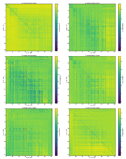
First, I want to note that in small transformers you see something not dissimilar! In some past experiments I analyzed the kernel of the query and key matrices for each attention head in GPT-2 and one of the smaller Gemma models, and found that attention head queries and keys share representation space only slightly more than would be expected by chance. Here’s the results from GPT-2 small:

| | |:–:|

In essence, what I did here was noted that per-head query, key, value, and output matrices are all low rank, since the head dimension is much lower than the model dimension. We can therefore use the left (right for output) singular vectors to compute the effective span of each component of the head. I then computed the Grassmannian distance between these vector spaces, and graphed it. As you can see, the diagonals are sort of visible—but not really that visible. Query matrices don’t look that much more like the corresponding head’s key matrices than they look like a random head’s key matrices—and that’s pretty weird! As a result, I wouldn’t invest that much into the argument about query and key asymmetry in TTT: they’re also asymmetric in full attention! There are exceptions, but by and large sequence mixing layers in large models are very complex. I think a notable deficit of this paper is that they didn’t include any comparitive results like this one: it’s hard to be sure how to interpret query/key asymmetry in TTT without knowing the corresponding facts about both linear and full attention. The authors argue that even without context, it disproves the key lookup/memorization interpretation of TTT, but I’m not so convinced that that was a widely held interpretation. It wasn’t my interpretation even before reading this paper, and so feels like a bit of a straw man. But I don’t work directly in this field, so perhaps the authors have a better finger on the pulse than I do.

4.4: Replacing queries with keys

As with section 4.2, the authors kindly clarified that these experiments were done by training fresh models.

While this is a fascinating and counter-intuitive result, it doesn’t necessarily scream linear attention to me. In standard attention, I agree that replacing queries with keys would result in a dramatic drop in performance, and it’s surprising that TTT seems immune to this. But to fully make the claim, we would also need to analyze linear attention networks. As we noted above, linear attention networks have separate queries and keys, and I would have expected keeping these distinct was necessary for performance—though perhaps that isn’t the case, as Liu et al. demonstrate for TTT! But the linear attention case is definitely unproved on the basis of the provided data.

I do think it’s very interesting that you can get away with using the same vectors for the queries and the keys in TTT, and I would not have guessed that this would work—so lots of credit belongs to the authors in considering performing this ablation. It very cleanly disproves the encyclopedia theory of KV binding, as pure look-up with this set-up would make sequence mixing pretty much impossible in the architecture. Ultimately, I think I’m mostly just impressed by the power of gradient descent though—the fact that the outer loop is able to adapt to this particular reduction in parameters shows just how powerful and flexible the inner loop gradient descent algorithm is, and the incredible ability of the outer loop to manipulate the inner loop’s algorithm. This result also seems almost at polar odds with the distributional asymmetry observed above, and I’m not entirely sure what to make of that.

Extended ablations on TTT components

The authors proceed to show that many components of TTT can be removed without performance hits. The most performant of their ablations replaces \(\phi_t\) from being an inner-loop parameter to being an outer-loop parameter. This returns us to linear attention, but with a nonlinear learnable kernel, which is certainly an interesting variant!

If Liu et al.’s results are to be believed, not only is it an interesting variant, it’s more powerful than baseline TTT systems—or, I would guess, more stable. I think a really serious problem that TTT has is that stochastic gradient descent over very small batches of data is simply not a very stable set-up. Taking up the algorithm analogy we made in the gradient ascent section, gradient descent is powerful—but theoretical guarantees on it likely don’t apply in the small data setting TTT operates in. I think Liu et al.’s results make a reasonably convincing argument that the expressivity gained by gradient descent is essentially wasted due to a lack of stability in the system, at least in the context of the analyzed architectures.

I don’t think this necessarily kills TTT as a field, though—gradient descent is still a powerful algorithm, and tuning that algorithm in stability-focused ways could continue to yield improvements. But it’s also worth taking a step back and asking what other inner loop algorithms are possible, with a specific eye on the bias/variance tradeoff in this low-data setting.

Conclusion: so what is TTT?

I’ve made it clear that I think there are notable and important differences between the formulations of TTT and linear attention. None of the empirical evidence I’ve seen really screams linear attention to me, and I disagree with the theoretical arguments made by Liu et al. But the question remains: since Liu et al. show that linear variants of analyzed TTT archtictures are as strong or stronger, what do we think TTT is actually doing?

While I think work remains to be done, and the two formulations are definitively \emph{mathematically} distinct, whether in practice TTT is approximately linear attention is something that I think is possible. The question is, does the \(\phi\) network change during inner loop updates? Or are the gradients that it receives essentially zeroed out due to vanishing gradients? This is another question that TTT researchers probably should address and study: how much are these nonlinear networks actually being updated in practice?

If in practice \(\phi\) is just bouncing around unstably, and the outer loop is essentially just trying to tend to the last layer, that would bring serious questions to current formulations of TTT, and whether it’s possible to truly scale beyond linear adaptation. It also might inform future TTT architectures: do we need to do some residual tricks to ensure gradients flow stably through the model, or would fancy optimizers solve some of these problems? Some of these experiments have already been done, but my experience with the TTT literature has mostly been evaluations of the downstream, outer loop performance. A very interesting future direction is to actually understand the way that the parameters of the inner loop \(f\) adapt to different contexts. Liu et al.’s experiment with changing \(\phi\) to be an outer loop parameter is an interesting first step in this direction, as a rather serious claim that \(\phi_\ell\) isn’t updating. But future research will be needed to confirm these results, and more detailed studies of \(f\) will be fascinating to see.

In terms of the “paradoxes” noted by Liu et al., it’s worth going back to the reason that gradient descent is involved with TTT in the first place: given any parametric function used for sequence mixing, in order to update it as new data arrives you need to apply some kind of algorithm. If you’re working with a neural net, gradient descent or gradient ascent are by far the most natural algorithms, as they naturally yield dense updates to the parametric function given low rank inputs. But for all that they’re convenient, that doesn’t mean that gradient descent is optimal. This is what I liked most from Liu et al.’s paper: gradient descent is the easiest available algorithm, but it might not be stable enough to keep. But that doesn’t mean we have to give up on the core concept of TTT: rather, we should be looking for other ways to iteratively update functions that don’t suffer from the same degree of instability.